

Introduction
Tap into the full potential of data analysis and revolutionize your career in an instant! If you are thinking that Excel can only help you do basic things like make simple grids and carry out sums, then you need to think again! Our guide will open up the doors to unlock all sorts of premium techniques such as dynamic VLOOKUPs, automatic macros and PivotTables, and more. No matter what industry you are in, whether it be business finance or marketing analytics, you’ll gain all sorts of time-saving insights by learning them.tions, and practical knowledge of Excel functions, macros, and data visualization. As businesses rely on data-driven decisions, demand for professionals with strong Excel skills continues to grow, offering promising career prospects.
Advanced Excel Tutorial for Beginners
The ultimate guide for beginners covers the gap from simple data entry to more advanced data management. We will cover all the essentials of advanced Excel with real-life examples, data structures, and automation scripts.
1. Advanced Formula Logic
To become an advanced Excel user, it is important to understand the logic of advanced formulas. Advanced formulas don’t operate on single cells only but examine the whole array (cells range), consider many criteria, and change themselves depending on the user actions.
Multi-criteria logics: SUMIFS and COUNTIFS
Basic SUMIF and COUNTIF formulas work with only one criterion. In a professional environment, you always need to work with several criteria. For example, you would like to know not only your total revenue, but the Total Revenue of “Spices” in “Chennai”.
The formula SUMIFS should start with the sum range, followed by pairs of criteria ranges and conditions:
SUMIFS(sum_range, criteria_range1, criteria1, [criteria_range2, criteria2]
If you want to calculate the total revenue specifically for Spices sold in Chennai, your advanced formula would look like this:
=SUMIFS(E2:E6, B2:B6, “Spices”, C2:C6, “Chennai”)
How it executes: Excel scans B2:B6 for “Spices” and C2:C6 for “Chennai”. It finds rows 2 and 5 (TXN001 and TXN004) match both conditions, and then adds their revenue together ($4,500 + $2,700) to return $7,200.
Nesting Logical Functions: IF, AND, OR
Nesting allows you to map out intricate business rules. Imagine you want to flag transactions that require a premium follow-up. The rule is: If a transaction is in Chennai AND the revenue is greater than $4,000, mark it as “High Priority”. Otherwise, mark it as “Standard”.
=IF(AND(C2=”Chennai”, E2>4000), “High Priority”, “Standard”)
By wrapping AND inside the logical test of an IF statement, Excel evaluates both conditions before returning a value.
2. Next-Generation Data Lookup: Beyond VLOOKUP
For many years, VLOOKUP ruled the world of data lookup. Yet, there are two main disadvantages associated with this function. First, VLOOKUP allows looking up data only from left to right; second, it becomes useless as soon as you add one more column to your sheet.
More sophisticated Excel users use INDEX and MATCH formulas and the advanced function XLOOKUP (included in modern versions of Excel).
The Power of XLOOKUP
XLOOKUP simplifies data retrieval by separating the lookup array from the return array. It looks up a value regardless of which side the return column lives on, and it defaults to an exact match.
XLOOKUP(lookup_value, lookup_array, return_array, if\_not_found}, match_mode]
Consider this separate Product Master Sheet:
| Product SKU | Product Name | Base Cost ($) |
| SK-SP01 | Spices | 12 |
| SK-TL02 | Tea Leaves | 18 |
| SK-CB03 | Coffee Beans | 22 |
The Classic Bulletproof Duo: INDEX and MATCH
If you are working on legacy workbooks or older Excel versions, INDEX and MATCH is your go-to configuration.
- MATCH finds the position number of an item in a list.
- INDEX returns the value at a specific position number inside a range.
When you nest them, MATCH tells INDEX exactly which row to look at:
=INDEX(B2:B4, MATCH(“SK-SP01”, A2:A4, 0))
Because you explicitly define the exact columns for searching and returning, this formula uses less processing power on massive datasets and never breaks when new columns are added.
3. Dynamic Array Formulas: The Modern Engine
One of the most revolutionary features of modern Excel is Dynamic Arrays. Rather than writing a formula and then copying it across a thousand rows, now you can write just one formula into a single cell, which will automatically “spill” down to other cells.
FILTER Function
The FILTER function helps you filter out an entire array of data according to a condition without interfering with the original table.
FILTER(array, include, [if_empty])
With the help of our original transaction table, all you need to do to obtain all those records where the number of units is more than 100 is to use this simple formula in an open cell:
=FILTER(B2:E6, D2:D6>100, “No records found”)
As a result, you will receive a dynamic table containing data about transactions with Spices (150 units) and Coffee Beans (120 units). The moment you enter a new record into your table, it will be added automatically.
The UNIQUE and SORT Functions
Cleaning dirty data frequently involves removing duplicates and organizing things alphabetically or numerically. Dynamic arrays handle this instantly.
To get a clean, unique list of all regions where you currently do business:
=UNIQUE(C2:C6)
Output: Chennai, Bangalore
To instantly sort that unique list alphabetically:
=SORT(UNIQUE(C2:C6))
4. Analytical Data Engines: Advanced PivotTables
While formulas are the brawn of Excel, the brain is the PivotTable. It takes several thousand rows of messy transactions and instantly summarizes them into an organized tabular form.
Step-by-Step Guide for Creating Advanced Summaries
- Go to any cell within your data table.
- Goto Insert > PivotTable.
- Select New Worksheet and click OK.
- In the Pivot Table Fields window, drag the Region field to Rows.
- Drag the Product field to Columns.
- Drag the Revenue field to Values.
Your entire worksheet becomes a matrix showing how much revenue each product made in each individual region:
| Row Labels | Coffee Beans | Spices | Tea Leaves | Grand Total |
| Bangalore | $0 | $6,000 | $2,400 | $8,400 |
| Chennai | $4,800 | $7,200 | $0 | $12,000 |
| Grand Total | $4,800 | $13,200 | $2,400 | $20,400 |
Advanced Pivot Table Tools: Calculated Fields & Slicers
- Calculated Fields: It is not required for you to introduce additional columns into your source data when calculating new figures. Within the PivotTable Analyze tab, choose Fields, Items, & Sets and then select Calculated Field. Create a new field named “Tax” through the formula =Revenue * 0.18.
- Slicers: They are the visual and interactive tools for filtering your Pivot Tables with just a single mouse click. Click on PivotTable Analyze, go to Insert Slicer, and check the box for Region.
5. Automated Mastery: An Introduction to VBA and Macros
An experienced Excel user should aim to avoid repetitive multi-step tasks that are time-consuming. When you receive a report every week and spend up to 20 minutes on cleaning headers, removing empty columns, and adding borders, all those actions can be automated using VBA (Visual Basic for Applications).
Firstly, you need to activate the Developer tab. To do this, go to File > Options > Customize Ribbon and tick the Developer checkbox.
The Macro Recorder
The simplest way to learn how to code is to have Excel do the coding for you.
- Select “Record Macro” from the Developer tab.
- Name the macro FormatReport and give it a shortcut key if you wish.
- Do your formatting (bold headers, font sizes, etc.).
- Then click on “Stop Recording.”
- This will automatically generate code based on your actions.
Writing VBA Code for Your Custom Needs
In order to open and write your scripts, simply click on Visual Basic located in the Developer tab (ALT + F11). Insert a new module (Insert > Module), and then use the following ready-to-run scripts.
Script 1: Automatically Autofit Columns and Turn On Gridlines
This macro will immediately select your current active sheet, remove any problems with text formatting, auto-fit all columns to avoid ### errors, and turn gridlines on.
Sub CleanAndFormatSheet()
Dim ws As Worksheet
Set ws = ActiveSheet
With ws
‘ Optimize Excel performance during execution
Application.ScreenUpdating = False
‘ Ensure gridlines are visible to the user
ActiveWindow.DisplayGridlines = True
‘ Target the used range to autofit column widths and row heights
.UsedRange.Columns.AutoFit
.UsedRange.Rows.AutoFit
‘ Format the first row as a clean, professional header block
With .Range(“A1”, .Cells(1, .Columns.Count).End(xlToLeft))
.Font.Bold = True
.Interior.Color = RGB(240, 240, 240) ‘ Soft Gray Background
.Borders(xlEdgeBottom).LineStyle = xlContinuous
.Borders(xlEdgeBottom).Weight = xlThin
End With
Application.ScreenUpdating = True
End With
MsgBox “Sheet formatting and clean-up complete!”, vbInformation, “Success”
End Sub
Script 2: Automatic Export of Excel Sheet to PDF
This script eliminates the need for menu-clicking each time you want to export a report by saving the current sheet as a PDF file in the same folder where the workbook is saved.
Sub ExportActiveSheetToPDF()
Dim ws As Worksheet
Dim wb As Workbook
Dim filePath As String
Dim fileName As String
Set ws = ActiveSheet
Set wb = ThisWorkbook
‘ Check if the workbook has been saved to give it a file path
If wb.Path = “” Then
MsgBox “Please save your Excel workbook first before exporting to PDF.”, vbCritical, “Error”
Exit Sub
End If
‘ Construct file paths dynamically
fileName = ws.Name & “_” & Format(Now, “YYYYMMDD_HHMMSS”) & “.pdf”
filePath = wb.Path & “\” & fileName
‘ Export the current sheet layout using standard PDF configurations
On Error GoTo ErrorHandler
ws.ExportAsFixedFormat _
Type:=xlTypePDF, _
Filename:=filePath, _
Quality:=xlQualityStandard, _
IncludeDocProperties:=True, _
IgnorePrintAreas:=False, _
OpenAfterPublish:=True
Exit Sub
ErrorHandler:
MsgBox “Failed to export PDF. Ensure the file isn’t currently open elsewhere.”, vbExclamation, “Export Failed”
End Sub
6. Advanced Data Hygiene: Power Query
In case of big datasets or disorganized ones, most of your time goes into cleaning up the data format errors. Power Query is the built-in Excel data transformation tool that can help address this issue once and for all.
With Power Query, there is no need to enter formulas to clean up the text and tables. The tool captures the data cleaning process and performs it automatically.
Text Transformation via Power Query
Consider that a client gives you a list in which customers’ names appear as bright, DR. BRIGHT, or RGB. Spacing is unpredictable; the capitalization is all wrong.
Instead of struggling with a formula such as =TRIM(PROPER(A2)), you have another option: process the data through Power Query.
- Select your data and click on the Data tab.
- Then click on From Table/Range to launch the Power Query Editor interface.
- Right-click on the column header for your problematic text.
- Choose Transform > Trim from the menu to remove all those pesky spaces right away.
- Right-click the column header once more and choose Transform > Capitalize Each Word.
How to Combine Multiple Datasets Without a Formula
Power Query is capable of joining tables as a relational database would do. In case you have a table with sales data in one tab and a master table with addresses in another, you will be able to combine your tables using the Merge Queries tool. It connects your columns by putting together a visual alignment of them and creating a perfect union of your data without using any XLOOKUP or VLOOKUP formula at all. When your transformations match perfectly, click on Close & Load.
Overview
Becoming an advanced Excel user is not a hit-or-miss journey; it is a step-by-step process. Make use of this framework as your strategic checklist to become proficient at each of these workflows:
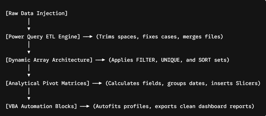
By avoiding the inefficiencies associated with manual and slow procedures, you will make fewer mistakes, save lots of time spent on repetitive tasks, and easily become a data expert.
Conclusion
Now you have begun your journey from being just a spreadsheet beginner to becoming an actual data specialist. With the help of learning not only how to use basic data entry but also how to utilize powerful functions, dynamic arrays, automated VBA scripts, and PivotTables, you already have the key building blocks that will allow you to transform your chaotic datasets into valuable insights for your company.
Please keep in mind that knowing Excel means not having to remember every single function; it means changing your approach to efficiency and automation. With all of the scripts mentioned above, you can easily get rid of numerous hours of tedious work.
If you are ready to accelerate your career development, get your resume-enhancing certification, and study from industry expert corporate trainers, it’s time to move forward with India’s best IT training portal. Join our Professional Advanced Excel Certification Course Now and make the leap from spreadsheet user to data strategy leader!